Simulation Design
Multi-generational pedigree
The simulation generates G_sim total generations:
G_sim - G_pedare burn-in generations (simulated but not recorded)G_pedgenerations are recorded in the pedigree- The last
G_phenoofG_pedare phenotyped
Each generation contains N individuals. With default settings
(\(N = 100{,}000\), \(G_{ped} = 6\)), the recorded pedigree contains
approximately \(600{,}000\) individuals.
Mating and reproduction
In each generation, couples are formed from the potential parent pool according to the following rules:
- An individual may participate in multiple couples.
- Males and females are paired randomly by default, or assortatively
on liability via
assort1andassort2. - Offspring are distributed across matings by a multinomial draw.
- Population size is held constant; some couples produce no offspring.
- MZ twins are assigned to matings with two or more offspring.
At default settings (mating_lambda = 0.5), approximately 77% of
individuals have a single partner and 23% have two or more, producing
a natural mix of full sibs, maternal half-sibs, and paternal half-sibs.
Pedigree relationship types
PedigreeGraph (from the pedigree-graph package) extracts 23 relationship
categories from simulated pedigrees using sparse matrix algebra. Each type is
parameterised by (up, down, n_ancestors) -- meioses up from individual A to
common ancestor(s), meioses down to individual B, and whether the link is
through 1 (half/lineal) or 2 (full, mated-pair) ancestors. Kinship is
\(n_{\text{ancestors}} \times (1/2)^{(\text{up} + \text{down} + 1)}\).
| Code | Label | Up | Down | Ancestors | Kinship | Degree |
|---|---|---|---|---|---|---|
| MZ | MZ twin | — | — | — | 1/2 | 0 |
| MO | Mother-offspring | 1 | 0 | 1 | 1/4 | 1 |
| FO | Father-offspring | 1 | 0 | 1 | 1/4 | 1 |
| FS | Full sib | 1 | 1 | 2 | 1/4 | 1 |
| MHS | Maternal half sib | 1 | 1 | 1 | 1/8 | 2 |
| PHS | Paternal half sib | 1 | 1 | 1 | 1/8 | 2 |
| GP | Grandparent | 2 | 0 | 1 | 1/8 | 2 |
| Av | Avuncular | 1 | 2 | 2 | 1/8 | 2 |
| GGP | Great-grandparent | 3 | 0 | 1 | 1/16 | 3 |
| HAv | Half-avuncular | 1 | 2 | 1 | 1/16 | 3 |
| GAv | Great-avuncular | 1 | 3 | 2 | 1/16 | 3 |
| 1C | 1st cousin | 2 | 2 | 2 | 1/16 | 3 |
| GGGP | Great²-grandparent | 4 | 0 | 1 | 1/32 | 4 |
| HGAv | Half-great-avuncular | 1 | 3 | 1 | 1/32 | 4 |
| GGAv | Great²-avuncular | 1 | 4 | 2 | 1/32 | 4 |
| H1C | Half-1st-cousin | 2 | 2 | 1 | 1/32 | 4 |
| 1C1R | 1st cousin 1R | 2 | 3 | 2 | 1/32 | 4 |
| G3GP | Great³-grandparent | 5 | 0 | 1 | 1/64 | 5 |
| HGGAv | Half-great²-avuncular | 1 | 4 | 1 | 1/64 | 5 |
| G3Av | Great³-avuncular | 1 | 5 | 2 | 1/64 | 5 |
| H1C1R | Half-1st-cousin 1R | 2 | 3 | 1 | 1/64 | 5 |
| 1C2R | 1st cousin 2R | 2 | 4 | 2 | 1/64 | 5 |
| 2C | 2nd cousin | 3 | 3 | 2 | 1/64 | 5 |
The max_degree parameter controls extraction depth (default 2, covering
through 1st cousins). Degree 3–5 types require deeper matrix products and
are computed only when requested. The registry is importable as
REL_REGISTRY and PAIR_KINSHIP from pedigree_graph.
Inbreeding and exact kinship
By default, kinship values are computed from the (up, down, n_ancestors)
formula, which assumes no inbreeding. When estimate_inbreeding: true is set
in config, PedigreeGraph computes exact inbreeding coefficients and pairwise
kinship using sparse matrix propagation:
-
compute_inbreeding()builds the kinship matrixKgeneration by generation using sparse products (P_g @ Kfor cross-generation,K_cross @ P_g.Tfor within-generation). The inbreeding coefficientF_i = K[mother_i, father_i]is extracted each generation. For non-consanguineous pedigrees (allF = 0), both functions short-circuit instantly. -
compute_pair_kinship(pairs)looks up exact kinship for each extracted pair from the cached sparseKmatrix. When inbreeding is present, kinship values deviate from the nominal formula by a factor of \((1 + F_a)\) where \(F_a\) is the inbreeding coefficient of the common ancestor.
| Pedigree | compute_inbreeding |
compute_pair_kinship |
Total |
|---|---|---|---|
| N=10K, 6 gens (60K individuals) | 12.9s | 2.3s | 15.2s |
| N=100K, 4 gens (400K individuals) | 11.9s | 0.9s | 12.7s |
Cost is dominated by the sparse P_g @ K products, which scale with the number
of nonzero kinship entries (i.e., the number of related pairs in the pedigree).
Fewer generations means sparser K and faster computation, even at larger N.
Pipeline stages
The simulation is conceptually split into four stages, plus downstream analysis:
- Simulate -- generate multi-generational pedigree with ACE liability components
- Phenotype -- map liability to age-of-onset via time-to-event models
- Censor -- apply age-window and competing-risk mortality censoring
- Sample -- optionally subsample and apply ascertainment bias
Followed by: validation, summary statistics, model fitting, and plotting.
Pipeline rule graph
The Snakemake rule graph showing how rules feed into each other:
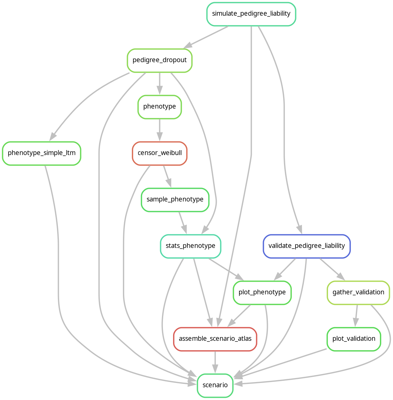
Regenerate the image after changes to the Snakefile or workflow rules:
The script writes docs/images/rulegraph.png. Pass an alternative target as
the first argument to render a different sub-DAG (default:
results/test/small_test/scenario.done).