Minimal ACE

The minimal configuration that exercises the full pipeline: two traits, no shared environment, no assortative mating, and the default phenotype model. The purpose is to verify that the simulator places variance where the configuration specifies, at two distinct heritabilities, before any deviation from the standard ACE model is introduced.

Configuration

The following block is added to config/examples.yaml:

minimal_ace:
  seed: 90001
  replicates: 1
  pedigree:
    trait1:
      A: 0.5
      C: 0.0
      E: 0.5
    trait2:
      A: 0.3
      C: 0.0
      E: 0.7

All other parameters (population size, generation counts, censoring, phenotype model) inherit from config/_default.yaml. Total variance is \(1.0\) for each trait, so the input heritabilities are \(h^2_1 = 0.5\) and \(h^2_2 = 0.3\). Both traits have \(C = 0\) and zero cross-trait correlation, so they constitute two independent calibration targets within the same simulation.

Run

snakemake --cores 4 results/examples/minimal_ace/scenario.done

Observations

The per-scenario atlas at results/examples/minimal_ace/plots/atlas.pdf contains two pages relevant to calibration. In each figure below the left panel corresponds to trait 1 (\(h^2_1 = 0.5\)) and the right panel to trait 2 (\(h^2_2 = 0.3\)).

Observation 1 — Realized \(h^2\) matches the input across generations

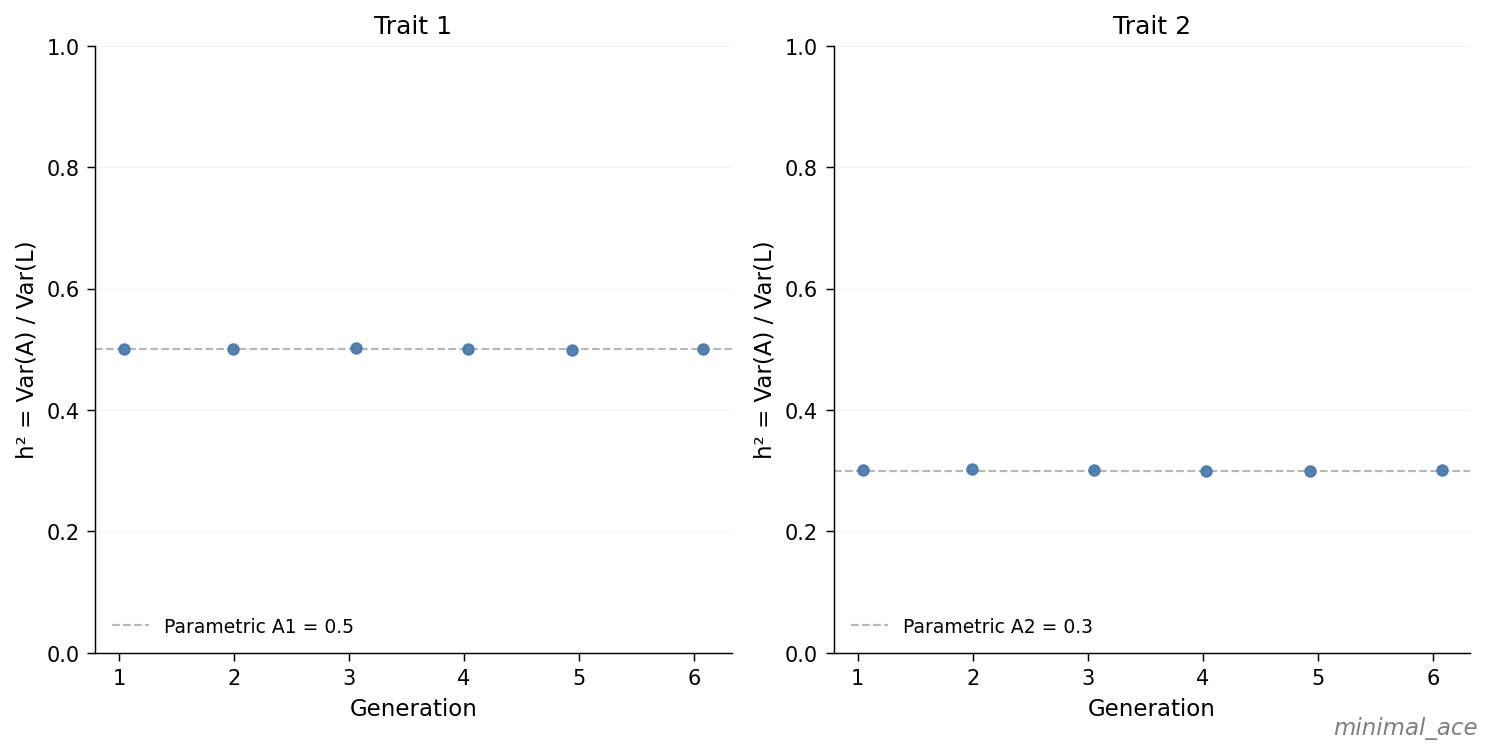
For each generation the realized \(\text{Var}(A) / \text{Var}(L)\) falls on the dashed parametric line at \(0.5\) (trait 1) and \(0.3\) (trait 2). In the absence of selection, assortative mating, and time-varying components, the variance ratio is invariant across generations, in agreement with the configured input.

Observation 2 — Liability correlations match ACE expectations across relative classes

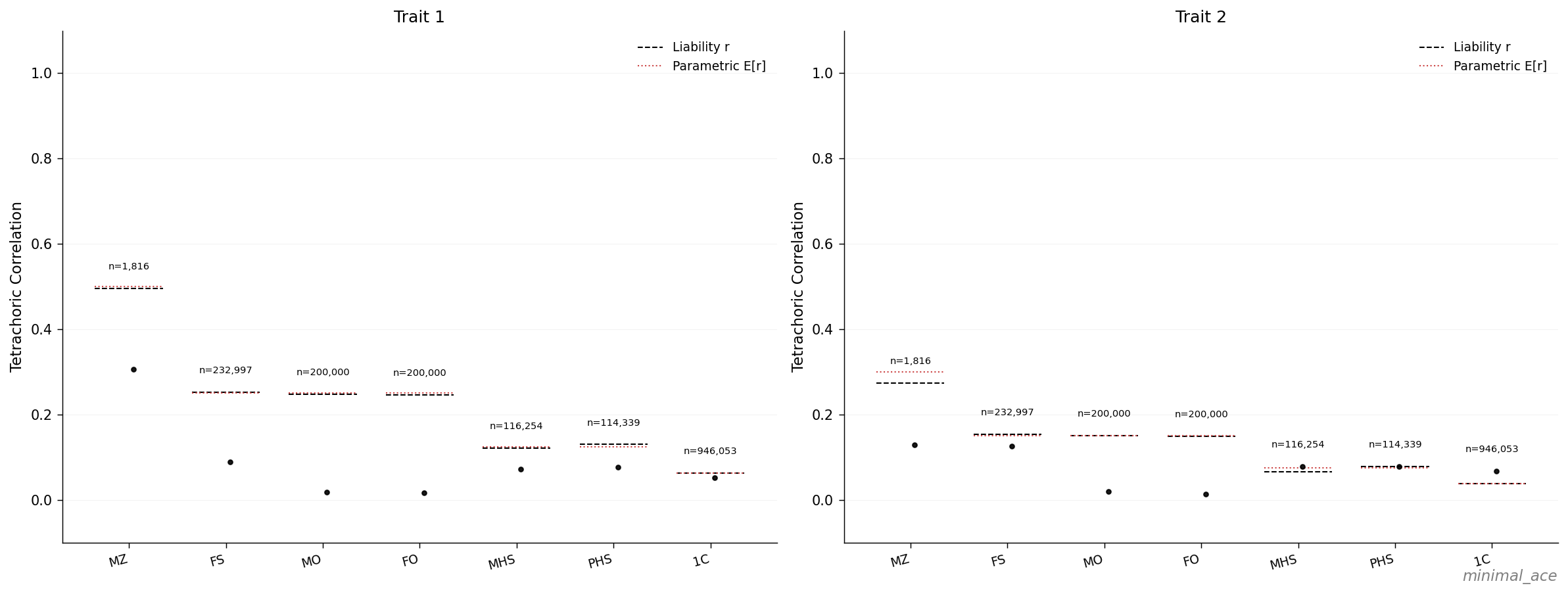
In both panels, the dashed liability-\(r\) bars coincide with the dotted parametric expectations across all seven relative classes:

Class	Trait 1 (\(h^2 = 0.5\))	Trait 2 (\(h^2 = 0.3\))
MZ	\(\approx 0.50\)	\(\approx 0.30\)
FS, MO, FO	\(\approx 0.25\)	\(\approx 0.15\)
MHS, PHS	\(\approx 0.125\)	\(\approx 0.075\)
1C	\(\approx 0.0625\)	\(\approx 0.0375\)

Each entry equals the relatedness coefficient (1, ½, ¼, ⅛) multiplied by \(h^2\). The MZ–FS gap equals \(h^2/2\) in both panels, corresponding to the quantity that Falconer's formula \(2(r_{MZ} - r_{FS})\) doubles in order to recover \(h^2\).

MZ is the limiting class for twin-based heritability estimators: at \(N = 100{,}000\) and a twin rate of \(\approx 0.012\), only \(n \approx 1{,}800\) MZ pairs are available, compared with \(n \approx 230{,}000\) full-sib pairs. As a result, the single-replicate MZ–FS Falconer estimate in validation.yaml is visibly noisier than the realized \(h^2\) in Observation 1, even though both target the same quantity.

The black dots are tetrachoric correlations computed on binary affected status under the default Weibull frailty phenotype model. They sit systematically below the liability-\(r\) bars because the Weibull frailty model lacks an explicit threshold structure; this regime is treated separately in Observed vs Liability h².

Summary

Variance components are recovered, the relative-pair correlation structure matches ACE expectations, and Falconer's identity holds in expectation, simultaneously at two distinct heritabilities. Subsequent examples introduce specific deviations from this baseline: a non-zero shared-environment component (Adding shared environment (C)), assortative mating (AM and Heritability), alternative phenotype models (Observed vs Liability h²), and time-varying \(E\) (Time-varying E and h² drift).

The full set of output files produced by one run is described in Output Structure.