Assortative mating and heritability¶

Assortative mating (AM) describes a pattern in which mates are more similar on some trait than would be expected by chance. Positive AM on a heritable trait couples the trait's genetic values across mates, and the coupling propagates to offspring. Across generations this reshapes the population's additive genetic variance, the correlations between relatives, and any quantity an investigator estimates from those correlations. This page presents three distinct manifestations of the effect in simACE output across a single set of scenarios.

The ACE Model page explains the variance decomposition used throughout.

Scenarios¶

All three scenarios use a lognormal cure-frailty phenotype model on trait 1 (model: cure_frailty, distribution: lognormal, mu=3.5, sigma=0.7, beta=1.0, beta_sex=0.0, prevalence=0.1), identical variance inputs (A=0.5, C=0.0, E=0.5 for trait 1 — no shared-environment component and no sex effect on hazard, so the story stays about vA vs vE), and differ only in the AM coefficient on trait 1.

Scenario	`assort1`	N	G_ped	G_pheno	G_sim	reps
`am_none`	0.0	100,000	10	10	10	3
`am_weak`	0.2	100,000	10	10	10	3
`am_strong`	0.4	100,000	10	10	10	3

Rebuild all three (and the comparison plots on this page) with:

snakemake --cores 4 examples_all

Observation 1 — AM inflates realized $v_A$ at equilibrium¶

The input values A=0.5, C=0.0, E=0.5 describe the variance decomposition in an idealized founder generation drawn under random mating: half of the liability variance is heritable, half is unique environment. Under positive AM, mates correlate on the genetic component of the liability. Standard quantitative-genetic theory shows that this correlation increases the between-locus linkage disequilibrium, and the population's realized additive variance grows over generations until a new equilibrium is reached. The realized $h^2 = v_A / (v_A + v_E)$ that any estimator should recover is therefore higher than the input $0.5$ — the estimator is not biased; the population itself has moved.

validation.yaml records the per-generation realized ACE components for every replicate, allowing this drift to be examined directly:

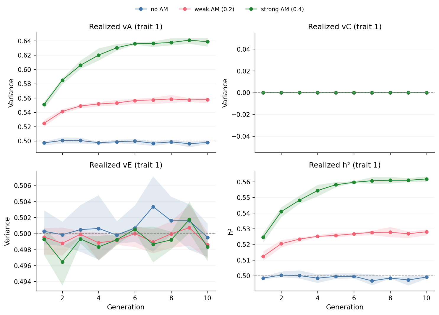
Realized variance components by generation, trait 1, across AM levels

Read the top-left panel first. The grey dashed line is the simulation input ($v_A = 0.5$). The am_none trace sits on that line across all 10 generations (sampling noise only). The am_strong trace drifts upward — each generation adds a small amount of shared genetic similarity between mates, and the cumulative effect on population vA is visible by generation 4–5 and stabilizes by generation 10. The am_weak trace sits in between.

The top-right panel ($v_C$) is a flat line at zero for all three scenarios, by construction: we set C = 0 so the story is cleanly about how AM redistributes variance between A and E. The bottom-right panel turns $v_A$ and $v_E$ into realized $h^2$: because $v_E$ stays close to its input value, inflation of $v_A$ flows directly into inflation of $h^2$. The same input ACE parameters can produce materially different "true" heritabilities depending on the mating system.

The shaded band around each line is the min/max across the three replicates; it is tighter than a glance suggests, because at $N = 100{,}000$ per generation the sampling variance of $v_A$ is small.

The trajectory plot displays the variance components as time-series numbers. The same effect is visible as a change in the per-individual distributions at equilibrium. Pooling all individuals in the last five generations (gens 5–9), the distributions of the additive genetic component $A_1$ (top) and total liability $A_1 + C_1 + E_1$ (bottom) overlay across the three AM scenarios as follows:

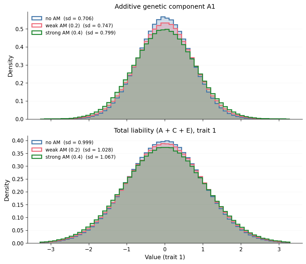
Distributions of A and total liability at AM equilibrium

Both panels widen from am_none → am_weak → am_strong. The top panel shows that AM directly stretches the additive genetic distribution; the standard deviations in the legend quantify the same inflation visible in the top-left panel of the trajectory plot. The bottom panel shows that the inflation in $A$ propagates directly to the total phenotype: because $C_1 = 0$ and $E_1$ is fixed by construction, the liability distribution widens by exactly the amount that $A_1$ does. Every panel in Observation 1 conveys the same fact, expressed once as a variance-component number and once as a distributional shape.

Observation 2 — AM distorts the similarity pattern among relatives¶

Observation 1 showed that AM moves the population's variance components. Observation 2 is the direct phenotypic consequence at the relative-pair level: AM also distorts the pattern of similarity across relatives, and the distortion differs depending on which slice of the pedigree is examined. This matters because most practical heritability estimators (twin-study Falconer, pedigree regressions, variance-component REML) rely on the structure of these correlations — they assume that the correlation between relatives of kinship $k$ is $k \cdot v_A + c \cdot v_C$. Breaking the structure causes silent drift in the estimator. Two views of the distortion follow: first a relationship-class summary (the inflation per kinship), then the raw joint distribution (the same inflation as a shape change in sib-pair liability space).

By relationship class¶

All correlations on this page are computed on the last five generations of each pedigree (generation >= G_pheno / 2, i.e. gens 5–9 for the G_pheno=10 configuration). By that point the AM-induced inflation of $v_A$ has approximately stabilized (see the trajectory plot in Observation 1), so this filter isolates equilibrium behavior from the early-generation transient. Pair extraction uses the full pedigree so that cousins of later-generation individuals can still be located via grandparents in earlier generations; only the correlation calculations themselves are restricted to the filtered subset.

Relative pairs are grouped into seven raw classes (MZ twins, full sibs, mother-offspring, father-offspring, maternal half sibs, paternal half sibs, first cousins). MZ twins are omitted from this chart: their liability correlation is pinned at $A + C$ regardless of AM, so they only crowd the y-axis. For the remaining classes, maternal and paternal pairs are pooled into a single PO and HS class, giving four classes on the x-axis below.

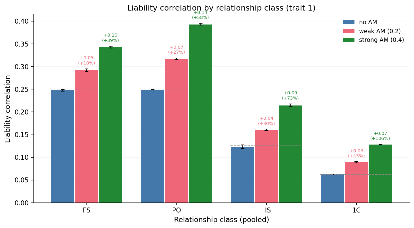
Liability correlation by pooled relationship class, across AM levels

The grey dashed lines are the random-mating expectations for the input $A = 0.5, C = 0$: $0.5 A$ for FS and PO, $0.25 A$ for HS, and $0.125 A$ for 1C. Above each non-baseline bar, a small label reports the absolute inflation ($\Delta r$) and the relative inflation (percent change) versus the am_none baseline for that relationship class, so that the qualitative pattern and the exact numbers can be read from the same chart. Reading the chart from left to right:

FS and PO both inflate under AM, and by visibly similar amounts — both hinge on a single shared parent-to-offspring transmission step, and AM inflates the additive variance that passes through it.
HS inflate too, but less — they share only one parent, so only one parent's AM-correlated genotype contributes to the shared liability.
1C inflate least in absolute terms but proportionally the most relative to their no-AM baseline.

A Falconer-style estimator takes two of these numbers, subtracts, and scales to obtain $h^2$. Under random mating, $h^2 \approx 2(r_{MZ} - r_{DZ})$ and $h^2 \approx 2 \cdot r_{PO}$ yield the same answer. Under AM they do not: $r_{MZ}$ is pinned, $r_{DZ}$ inflates, $r_{PO}$ also inflates, so the two formulas diverge — and neither recovers the realized $h^2$, which Observation 1 showed is itself moving.

As a joint-distribution shape change¶

The bar chart summarizes similarity as a single number per class. The same effect is visible as a change in the shape of the joint liability distribution of relatives. For full sibs, every non-twin full-sib pair is taken, the liabilities of the first two children per family (by id order) are sampled, and the bivariate distribution is summarized by two objects: the 2-SD covariance ellipse (approximately 95% of the density under a Gaussian fit) and the best-fit regression line of sib-B liability on sib-A liability. Founders are excluded (no parents); MZ twins are excluded (they would pile directly on $y = x$ by construction); the same last-five-generation filter as the bar chart above is applied, so that both views describe the AM equilibrium.

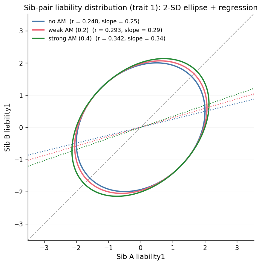
Sib-pair liability shape across AM levels

The chart overlays, on a single axis, three 2-SD covariance ellipses (approximately the 95% contour of the joint sib-pair liability distribution under a Gaussian fit) and the three best-fit regression lines of sib-B on sib-A, one per scenario. The grey dashed line is y=x. The legend labels each scenario with its Pearson $r$ and the slope of its regression line.

From am_none to am_strong, two effects grow in lockstep: the ellipse's long axis stretches further along the $y = x$ direction (the cloud becomes more elongated), and the regression line rotates upward (the slope increases from about $0.25$ at random mating to about $0.34$ under strong AM). A steeper slope means that a sibling above the mean predicts a larger above-mean deviation in the other sibling; this is the phenotypic fingerprint of the AM-inflated FS correlation shown in the bar chart above, and of the AM-inflated additive variance from Observation 1. The three views describe a single phenomenon; Observation 3 picks up the estimator-bias consequence.

Observation 3 — AM biases naive estimators that assume random mating¶

Observations 1 and 2 establish two failure modes under AM: the population's realized $v_A$ (and with it the realized $h^2$) has moved above the input value, and the correlations between relatives have inflated by a class-dependent amount. A "naive" heritability estimator — one that maps a single pedigree correlation (or regression slope) to $h^2$ under the assumption of random mating — is therefore guaranteed to mismatch the truth under AM. The remaining question is by how much, and in which direction, for each estimator.

Five textbook estimators are computed on each scenario:

Twin Falconer: $h^2 = 2 \cdot (r_{MZ} - r_{FS})$
Sibs only: $h^2 = 2 \cdot r_{FS}$
Midparent PO: $h^2 = $ slope of offspring liability regressed on mean of parent liabilities
Half-sibs: $h^2 = 4 \cdot r_{HS}$
Cousins: $h^2 = 8 \cdot r_{1C}$

Each of these estimators recovers $h^2$ under random mating. Under AM, each is contaminated by the AM-induced inflation of the correlation on which it depends, but by different amounts because the inflation per class differs (see Observation 2). As in Observation 2, all correlations, the midparent-offspring regression slope, and the realized-$h^2$ reference are computed on the last five generations of each pedigree (generation >= G_pheno / 2, i.e. gens 5–9 at G_pheno=10). This isolates the AM equilibrium. Pair extraction still uses the full pedigree so that cousins of later-generation individuals can be located via earlier-generation grandparents, and the midparent regression reads parent liabilities from the full pedigree even when the parents reside in earlier generations.

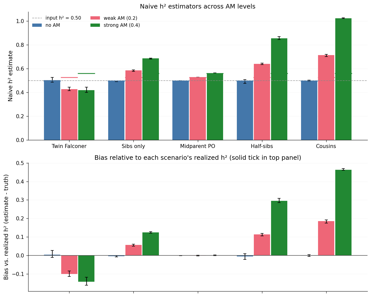
Naive h² estimates and bias vs. realized truth, across AM levels

The top panel shows each estimator's raw output per scenario. Short solid horizontal ticks, coloured to match each scenario's bars, mark that scenario's realized $h^2$ (the final-generation $v_A / (v_A + v_C + v_E)$ from Observation 1). The grey dashed line is the input $h^2 = 0.50$.

The bottom panel recasts the top as signed bias: each bar is the per-replicate estimator value minus that replicate's realized $h^2$, averaged across replicates. The horizontal line at zero corresponds to agreement with the realized truth; bars above zero overestimate, bars below underestimate.

By estimator¶

Three patterns are evident:

am_none calibrates cleanly. Every estimator coincides with the realized-$h^2$ tick in the top panel and shows near-zero bias in the bottom panel. The naive formulas behave as advertised when the random-mating assumption is satisfied.
Midparent-offspring regression is nearly AM-robust. Even under am_strong, the midparent-PO slope tracks the realized $h^2$ to within sampling tolerance. This is the classical result that the midparent-offspring regression recovers $h^2$ at equilibrium largely independent of mating structure, because the regressor already pools the two AM-correlated parental genotypes.
Cousin-only estimation explodes. With a multiplier of $8\times$, even the modest inflation of $r_{1C}$ under AM produces a large absolute bias: the strong-AM estimate approaches $1.0$, well above the realized $h^2 \approx 0.56$. Half-sibs ($4\times$) drift less than cousins but more than full sibs ($2\times$); the bias is monotone in the kinship multiplier.

Diagnostic signature¶

The divergence across estimators is itself the diagnostic signal of AM. When correlations are available across multiple kinship classes and yield mutually inconsistent $h^2$ estimates, the population is signalling that the random-mating assumption underlying the naive formulas is wrong. The practical implication of Observation 3 is that naive $h^2$ estimators appear sensible in isolation but are only trustworthy when their outputs agree; disagreement indicates that the kinship structure assumed by the estimator does not match the kinship structure of the population.