Observed-scale vs liability-scale heritability

In quantitative genetics, \(h^2 = v_A / (v_A + v_C + v_E)\) is defined on the liability scale — the continuous latent trait whose threshold crossings (or whose hazard trajectories) produce the observable phenotype. In real data the liability is almost never directly observed; the observable quantity is a binary affected / unaffected status, possibly with age of onset. Recovering liability-scale \(h^2\) from that observed signal requires an assumed mapping between the two, and the mapping depends on the phenotype model that generated the observation.

This page compares three phenotype models under otherwise-identical ACE truth in order to characterize when a tetrachoric-based estimator on binary data recovers liability-scale \(h^2\) and when it does not.

Scenarios

All three scenarios share:

• \(A_1 = 0.5\), \(C_1 = 0.0\), \(E_1 = 0.5\) → input \(h^2 = 0.5\)
• No assortative mating (assort1 = assort2 = 0)
• \(N = 100{,}000\) founders, \(G_{ped} = G_{pheno} = G_{sim} = 10\), 3 replicates
• Target prevalence \(K \approx 0.1\); observed \(K \approx 0.06\) in all three scenarios (comparable across models, which is what matters for the comparison)
• No sex effect on hazard (\(\beta_{sex} = 0\)), liability-to-hazard coupling \(\beta = 1.0\)

They differ only in the phenotype model family used to map the latent liability to an observed affection status:

Scenario	Model	Params
model_ltm	adult, method: ltm	cip_x0 = 16.3, cip_k = 0.376
model_cure_frailty_ln	cure_frailty, distribution: lognormal	mu = 3.5, sigma = 0.7
model_frailty_wb	frailty, distribution: weibull	scale = 2160, rho = 0.8

The LTM scenario is the classical liability-threshold model: an individual is affected iff their liability exceeds a sex-/age-specific threshold. The frailty scenarios instead treat liability as the log-hazard of an age-of-onset process; whether an individual is "affected" at the end of their observation window depends on liability and on time. Cure-frailty adds a susceptibility fraction on top: only a subset of individuals is at risk at all, and the hazard governs onset within that subset.

Rebuild all three (and every other docs-embedded comparison plot) with:

snakemake --cores 4 examples_all

Observation — Tetrachoric Falconer depends on the shape of the liability→observed map

Two estimators of \(h^2\) are applied to each scenario:

• Liability Falconer \(= 2 \cdot (r_{MZ}^{\text{liab}} - r_{FS}^{\text{liab}})\), computed on the continuous simulated liability. In real data this is not feasible because the latent trait is unobserved; here it plays the role of an oracle reference — the value the Falconer formula returns when supplied with the correct correlation inputs.
• Tetrachoric Falconer \(= 2 \cdot (r_{MZ}^{\text{tetra}} - r_{FS}^{\text{tetra}})\), computed from tetrachoric correlations on binary affected status. Tetrachoric assumes a bivariate-normal liability under a single threshold mapping; the accuracy of the resulting estimate depends on how well that assumption matches the data-generating process.

Specifically: under model_ltm and model_cure_frailty_ln, tetrachoric Falconer approximately recovers the realized \(h^2\). Under model_frailty_wb it severely underestimates, because pure frailty lacks the threshold structure — either a hard liability cutoff or a susceptibility fraction — on which tetrachoric depends.

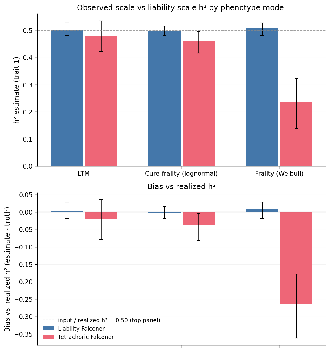
The top panel shows each estimator's raw output per scenario. The dashed grey line is the input \(h^2 = 0.50\); it doubles as the realized-\(h^2\) reference here because there is no AM to push the population off the input value (if realized had diverged, a short dark-grey tick would be drawn at its actual location for that scenario).

The bottom panel recasts the top as signed bias: each bar is the per-rep estimator value minus that rep's realized \(h^2\).

Interpretation

• Under LTM, liability-Falconer and tetrachoric-Falconer essentially coincide and both land within sampling noise of realized \(h^2\). This is the classical textbook result: when the data are generated by a liability-threshold model, tetrachoric on binary outcomes recovers the underlying continuous correlation structure and Falconer's formula yields the correct \(h^2\).
• Under cure-frailty, tetrachoric also recovers realized \(h^2\), with slightly more residual bias than LTM but of the same order of magnitude. The cure fraction — a hard susceptibility cutoff — acts as an implicit threshold on the liability, which is the regime for which tetrachoric was designed. A mixture model with a distinct at-risk / not-at-risk split is therefore LTM-like in this respect.
• Under pure Weibull frailty, tetrachoric drops to approximately half of realized \(h^2\). Without a cure fraction, every individual is at some risk and the affected indicator is a smooth, non-threshold function of liability (integrated hazard over an observation window). The smooth mapping compresses the correlation gap between MZ twins and full siblings: the underlying liability correlations match those of the other scenarios (\(r_{MZ} \approx 0.50\), \(r_{FS} \approx 0.25\)), but their tetrachoric projections onto binary status are much closer (\(r_{MZ}^{\text{tetra}} \approx 0.27\), \(r_{FS}^{\text{tetra}} \approx 0.15\)), yielding a low Falconer estimate.

Implications

Tetrachoric-based \(h^2\) estimators assume the phenotype is a threshold function of a bivariate-normal liability. LTM satisfies this exactly, and cure-frailty satisfies it approximately (the susceptibility indicator is itself a threshold-like variable). For genuinely smooth age-of-onset traits with no distinguishable at-risk subgroup, the tetrachoric approach systematically under-estimates liability-scale \(h^2\). In that regime, an age-of-onset-aware method (PA-FGRS, EPIMIGHT, first-passage-time) is not optional but a necessary correction.