Time-varying E and h² drift

A core assumption of the standard ACE model is that the variance components are constants of the population — fixed numbers attached to the trait, inherited from generation to generation as if they were physical constants of the trait itself. They are not. Real environments shift across cohorts: education, urbanization, diet, screening practices, public-health interventions, and many other factors alter the typical magnitude of the non-genetic, non-shared-environment contribution to a trait. When the unique-environment variance \(v_E\) moves across generations, the realized heritability \(h^2 = v_A / (v_A + v_C + v_E)\) moves with it, even when \(v_A\) remains unchanged. This page describes the form of that drift in simACE output, its signature in within-cohort relative-pair correlations, the mis-aggregation incurred by a naive heritability estimator pooled across cohorts, and the role of the standardize configuration mode in determining whether observed-scale prevalence remains stable or drifts in lockstep.

The ACE Model page explains the variance decomposition. The AM and Heritability page covers a different way the population can deviate from its inputs (the mating system); this page treats the temporal axis instead. Both pages share the same fundamental warning: the input numbers and the realized numbers can disagree, and naive estimators do not signal which is being reported.

Scenarios

All eight scenarios use a liability-threshold (adult / method: ltm) phenotype model on trait 1 with cip_x0=16.3, cip_k=0.376, prevalence=0.1, beta=1.0, beta_sex=0.0, identical \(A_1=0.5\), \(C_1=0.0\), no AM, \(N=100{,}000\), \(G_{ped}=G_{pheno}=10\), 3 replicates. All scenarios start at \(E_1 = 0.5\) in generation 0, so the gen-0 founder state is identical across them.

The four E trajectories differ in how \(E_1\) moves across generations 0–9:

Trajectory	\(E_1\) schedule (linear, gen 0 → gen 9)
e_flat	0.5 constant
e_rise_mild	0.5 → 0.6 (Δ = +0.1)
e_rise_steep	0.5 → 0.7 (Δ = +0.2)
e_fall_steep	0.5 → 0.3 (Δ = −0.2)

Each trajectory has a _std and _nostd variant with matched seeds: the simulated liability columns are byte-identical within a pair; only the binary affected status (in phenotype.parquet) differs. The _std scenarios use the legacy bool form standardize: true, which the config-load shim resolves to standardize: "global"; the _nostd scenarios use standardize: false (resolved to standardize: "none"). The third available mode, "per_generation", is discussed in Observation 4 below as the prevalence-flattening alternative. Observations 1–3 use the four _std scenarios because they concern the liability scale, where the standardize mode is invisible. Observation 4 contrasts _std against _nostd, since that contrast is precisely the observed-scale axis.

Rebuild all four (and the comparison plots on this page) with:

snakemake --cores 4 examples_all

Observation 1 — Realized \(v_E\) tracks the configured trajectory; \(h^2\) drifts with it

The simulator reads the per-generation \(E_1\) values from the configuration dictionary, draws independent normal noise of the corresponding variance for every individual in that generation, and adds it to the genetic component to form the liability. If the simulator behaves as specified, the realized \(v_E\) recovered from the per-individual liability columns should track the input schedule exactly; \(v_A\) should remain flat at the input \(0.5\) (no AM, no selection); and \(h^2 = v_A / (v_A + v_E)\) should drift inversely to \(v_E\).

validation.yaml records the per-generation realized ACE components for every replicate, allowing this drift to be examined directly:

(A note on gen indexing: simACE stores 0-indexed generations in pedigree.parquet (gens 0–9 for G_pheno=10) but labels them 1-indexed in validation.yaml (generation_1 … generation_10). The trajectory plot here reads validation.yaml so its x-axis is 1–10, with gen 1 = founders. The cohort plots later on this page (FS correlation, Falconer, components-by-generation) read pedigree.parquet, so their x-axis is 0–9 with gen 0 = founders. In both cases gen "\(N\)" is the same physical cohort under a different label; the figures just inherit the indexing of the file they read.)

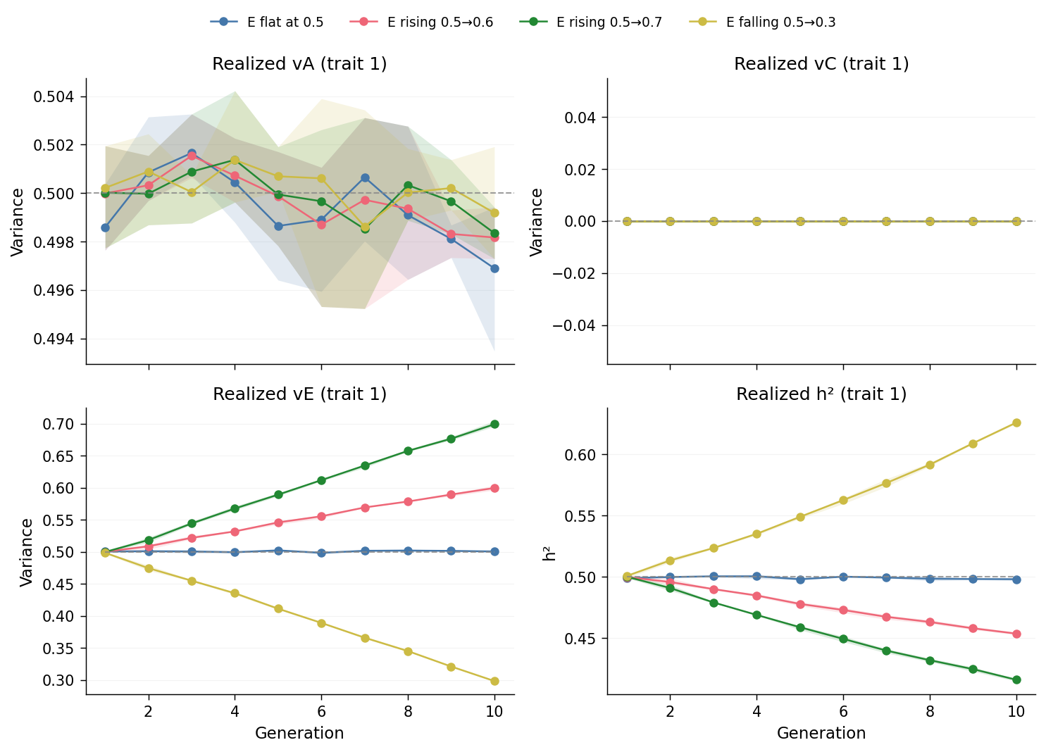
The bottom-left (\(v_E\)) panel: the horizontal grey dashed line at \(0.5\) is the e_flat reference schedule, drawn for visual calibration. Each solid trace tracks the scenario's configured schedule essentially exactly, with sampling noise smaller than the line thickness at \(N = 100{,}000\) per generation: e_flat is flat at \(0.5\), the rising scenarios climb in straight lines toward \(0.6\) / \(0.7\), and e_fall_steep declines symmetrically toward \(0.3\).

The top-left (\(v_A\)) panel is flat at \(0.5\) across every scenario, by construction: \(A\) is constant in the configuration and no AM or selection redistributes it. The top-right (\(v_C\)) panel is flat at zero, also by construction. Both confirm that the trajectory of \(v_E\) is the only component moving across generations.

The bottom-right (\(h^2\)) panel is the consequence: with \(v_A\) fixed and \(v_C = 0\), \(h^2 = 0.5 / (0.5 + v_E)\). Substituting the per-generation \(v_E\) values, the \(h^2\) trajectories form mirror images of the \(v_E\) panel. At the final generation:

• e_flat ≈ 0.500 (input, unchanged)
• e_rise_mild ≈ 0.455 (\(h^2\) fell by ~0.045)
• e_rise_steep ≈ 0.417 (\(h^2\) fell by ~0.083)
• e_fall_steep ≈ 0.625 (\(h^2\) rose by ~0.125)

The same input ACE parameters can therefore produce materially different "true" heritabilities across generations of a single population. This is purely a temporal/cohort effect, with no AM-like mechanism, no selection, and no environmental cross-transmission.

The trajectory plot displays the variance components as time-series numbers. The same effect is visible as a change in the per-individual distributions across generations. Sampling three representative cohorts (gen 1, gen 5, gen 9) and overlaying their distributions of \(A_1\) (top) and total liability \(A_1 + E_1\) (bottom):

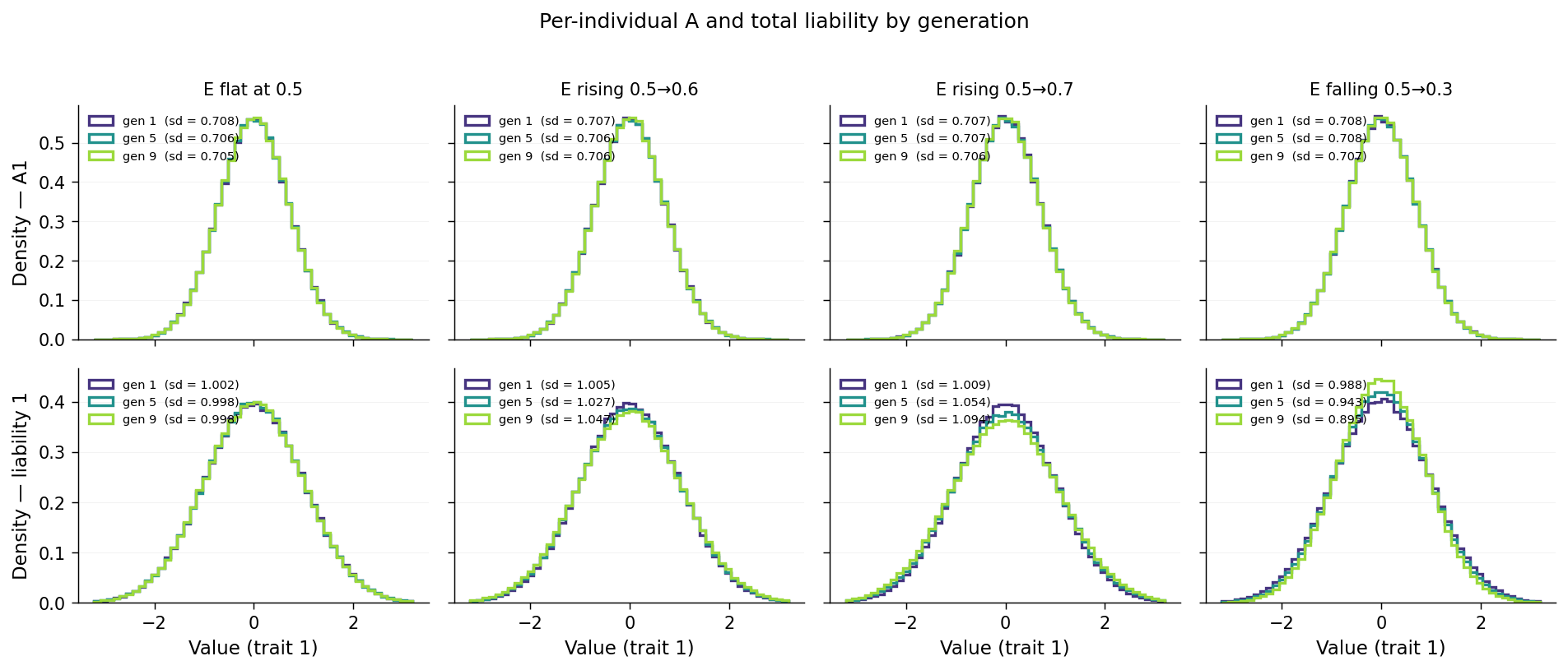
Top row (A) is the calibration check: \(A_1\) is constant by config, so all three generations should have indistinguishable distributions in every scenario. They do — SDs sit between 0.705 and 0.708 across all 12 (scenario × generation) cells in the top row, well within sampling noise.

Bottom row (total liability) is where the story is:

• e_flat: all three gen curves overlap at SD ≈ 1.00. No drift.
• e_rise_mild: gen 1 SD ≈ 1.005, gen 5 ≈ 1.027, gen 9 ≈ 1.047. Visible widening as later cohorts pick up more E variance.
• e_rise_steep: gen 1 ≈ 1.009 → gen 9 ≈ 1.094. Wider swing; the gen 9 curve is visibly flatter at the peak and fatter in the tails.
• e_fall_steep: gen 1 ≈ 0.988 → gen 9 ≈ 0.895. Reverse direction — the gen 9 curve is taller and narrower, because \(v_E\) has shrunk.

The widening (or narrowing) of the bottom-row distributions is the same phenomenon as the bottom-left \(v_E\) trace and the bottom-right \(h^2\) trace in the trajectory plot, expressed as a shape change in per-individual values rather than as a numerical trajectory.

Observation 2 — Within-cohort FS correlation depends on the generation of the pair

Observation 1 showed how the population's per-generation variance components shift. Observation 2 is the direct consequence at the relative-pair level: the expected correlation between full sibs born into a high-\(v_E\) cohort is lower than between full sibs born into a low-\(v_E\) cohort, because the non-shared-environment slice of the liability is independent within the sibling pair. The classical random-mating expectation \(r_{FS} = 0.5 \cdot v_A + v_C\) holds only when the population has a stable variance structure; with non-stationary \(v_E\), the FS correlation varies cohort by cohort.

The correlation on liability1 is computed between full-sib pairs in which both members reside in the same generation \(g\). Founders are excluded (they have no parents, hence no FS pairs); MZ twins are excluded by construction (simace/core/pedigree_graph.py:_sibling_pairs filters on twin == -1). The per-replicate \(r_{FS}(g)\) is averaged across the three replicates, with min/max shaded as the envelope.

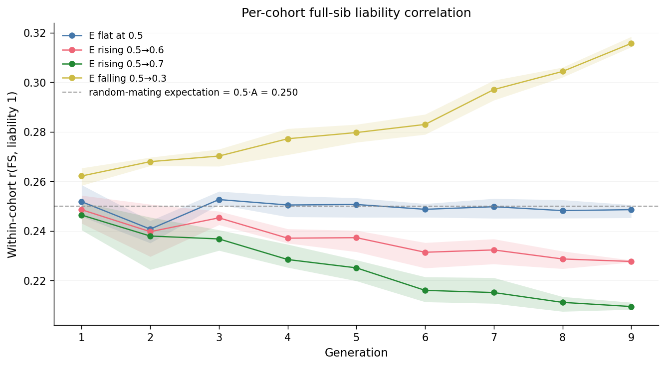
The grey dashed line at \(0.250\) is the random-mating expectation \(0.5 \cdot A_1 + C_1 = 0.5 \cdot 0.5 + 0 = 0.25\), matching the value used in the AM page. Reading each line:

• e_flat is flat at \(\approx 0.250\) across all generations 1–9. This is the calibration: when \(v_E\) does not move, neither does the FS correlation, exactly as the standard model predicts.
• e_rise_mild starts near \(0.249\) in gen 1 and declines monotonically to \(\approx 0.228\) by gen 9. The slope is shallow because the \(v_E\) swing is shallow (\(\Delta = +0.1\)).
• e_rise_steep declines from \(\approx 0.246\) to \(\approx 0.210\) by gen 9; the drop is roughly twice the magnitude of e_rise_mild, mirroring the doubled \(v_E\) swing (\(\Delta = +0.2\)).
• e_fall_steep moves in the opposite direction, climbing from \(\approx 0.262\) at gen 1 to \(\approx 0.316\) by gen 9.

The endpoint values match the analytic prediction \(r_{FS} = 0.5 \cdot v_A / (v_A + v_E)\) to within sampling noise: at \(v_A = 0.5\), \(v_E = 0.7 \Rightarrow r_{FS} = 0.208\) (steep rise); at \(v_E = 0.3 \Rightarrow r_{FS} = 0.313\) (steep fall).

This is the statistical signature of cohort effects on heritability. A pedigree-correlation analysis that pools full sibs across generations and reports a single \(r_{FS}\) averages over these moving cohorts; the returned value is a population-weighted average of cohort-specific truths, not the truth of any single cohort.

Observation 3 — Pooled-across-generations naive Falconer matches no generation's truth

Observation 2 established the within-cohort signal; Observation 3 concerns the consequence when the cohort axis is ignored and the pooled relative-pair correlations are inserted into the standard Falconer formula \(h^2 = 2 \cdot (r_{MZ} - r_{FS})\). Within each cohort, Falconer is well-calibrated: \(r_{MZ}\) within gen \(g\) is approximately \(v_A / (v_A + v_E^{(g)})\), equal to the realized \(h^2(g)\); \(r_{FS}\) within gen \(g\) is approximately \(0.5 \cdot v_A / (v_A + v_E^{(g)})\); and their difference scales correctly. Pooling MZ and FS pairs across all generations smears the moving truth into a single number that depends on generation-population weights but matches no individual generation's \(h^2\).

The pooled-across-generation Falconer estimate is computed on the full pedigree (every individual, every generation) for each replicate, and compared to the per-cohort Falconer estimates and the per-cohort realized \(h^2\):

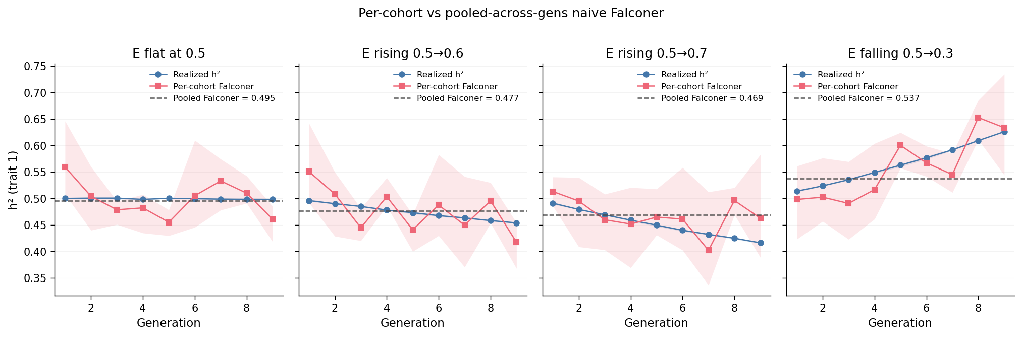
Each panel corresponds to one trajectory. The blue line is the per-cohort realized \(h^2\) from Observation 1 (the truth). The rose-coloured line is the per-cohort Falconer estimate (computed within the cohort using \(r_{MZ}\) and \(r_{FS}\) on individuals in that generation). The dark dashed horizontal line is the pooled-across-generation Falconer estimate.

Reading each panel:

• e_flat: per-cohort Falconer tracks per-cohort realized \(h^2\) at \(\approx 0.50\), and the pooled Falconer dashed line coincides with both. No cohort drift, no pooling artefact: the standard model recovers the truth.
• e_rise_mild and e_rise_steep: the per-cohort lines decline in lockstep across generations; the pooled Falconer dashed line falls in the middle of the per-cohort range, matching no individual generation's truth. For e_rise_steep the pooled estimate lands at \(\approx 0.469\), between gen-1's truth (\(\approx 0.49\)) and gen-9's truth (\(\approx 0.42\)); for e_rise_mild the pooled estimate is \(\approx 0.477\), between truths of \(\approx 0.50\) and \(\approx 0.45\).
• e_fall_steep: per-cohort lines climb across generations; the pooled Falconer estimate (\(\approx 0.537\)) sits between gen-1's truth (\(\approx 0.51\)) and gen-9's truth (\(\approx 0.625\)), confirming direction symmetry.

The per-cohort Falconer line is visibly noisier than the realized-\(h^2\) line because per-cohort \(r_{MZ}\) rests on only \(\approx 600\) MZ pairs at \(N = 100{,}000\) (twin rate \(\approx 0.012\)); the standard error on \(r_{MZ}\) is therefore meaningful at the per-generation scale even though it is negligible when pooled.

The diagnostic signal of cohort drift is the disagreement between per-cohort Falconer estimates across generations. When Falconer is estimated separately by birth-cohort decade and visibly different numbers result, the population is signalling that the random-stationarity assumption underlying a single pooled \(h^2\) is wrong for that population.

Observation 4 — standardize="global" offsets but does not flatten prevalence drift under the adult/LTM model

Observations 1–3 concern the liability scale, where the standardize mode is invisible (it affects only the mapping from liability to binary affected status). Observation 4 examines that mode explicitly. Under the adult / method: ltm phenotype model, the threshold is set as \(T = \Phi^{-1}(1 - K)\) where \(K\) is the configured prevalence. With standardize="global" (the default; equivalent to the legacy standardize: true), AdultModel._simulate_ltm standardizes liability to mean \(0\) and standard deviation \(1\) across the entire pedigree — not per-generation — before comparing to \(T\). With standardize="none" (legacy standardize: false), raw liability is compared to \(T\) directly. A third mode, standardize="per_generation", flattens the per-cohort drift entirely; see the subsection below.

The matched-seed pairs (e_*_std vs e_*_nostd) make the global-vs-none contrast exact: the pedigree and liability columns are identical within a pair, so any per-generation prevalence difference is purely due to the standardize choice.

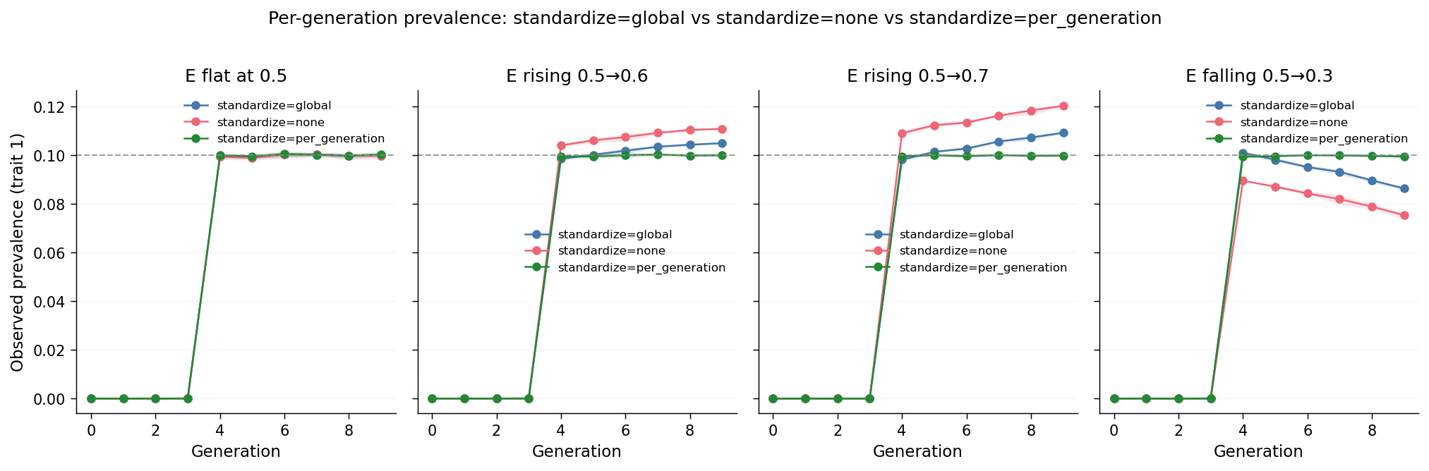
Each panel is one trajectory. Three lines per panel: standardize="global" (legacy true), standardize="none" (legacy false), and standardize="per_generation". The grey dashed line is the input \(K = 0.10\). The matched-seed e_*_std and e_*_nostd scenarios feed the first two lines; the new e_*_pergen scenarios (matched seeds again) feed the third.

The age-censoring artefact (gens 0–3)

In every panel both lines sit at exactly \(0\) for generations 0–3 and jump up at gen 4. This is not a bug; it reflects the LTM age-of-onset model. With cip_x0 = 16.3 and cip_k = 0.376, the cumulative incidence probability for a case is logistic with midpoint at age \(16.3\), so cases that would eventually onset do not manifest until approximately age 12 or later. The pipeline assigns each generation an age of observation that decreases for younger generations (gen 9 is "now", gen 0 is the oldest ancestor cohort); the youngest individuals have not aged into onset by their censor window and therefore appear 0%-affected even though their liabilities match those of their ancestors. Generations 4–9 should be read.

Effect of global vs none (gens 4–9)

• e_flat: both lines sit at \(\approx 0.100\) across gens 4–9. This is the calibration baseline; it matches the configured \(K = 0.10\) within sampling noise.
• e_rise_mild: standardize="global" rises \(0.099 \to 0.105\) (\(\Delta = +0.006\)); standardize="none" rises \(0.104 \to 0.111\) (\(\Delta = +0.007\)). The two slopes are nearly identical; "global" shifts the absolute level by \(\approx 0.005\)–\(0.006\) but does not reduce the per-generation drift.
• e_rise_steep: "global" \(0.098 \to 0.109\) (\(\Delta = +0.011\)); "none" \(0.109 \to 0.120\) (\(\Delta = +0.011\)). The same pattern obtains; the swing is larger than for e_rise_mild because \(v_E\) swings more.
• e_fall_steep: "global" \(0.101 \to 0.086\) (\(\Delta = -0.015\)); "none" \(0.090 \to 0.075\) (\(\Delta = -0.014\)). Direction symmetric; slopes again match but the offsets differ.

The key fact is that the slopes are essentially identical between _std and _nostd. The "global" mode adjusts the level of the per-generation prevalence — rising-\(E\) scenarios have lower prevalence under "global" because the cohort-wide standardization scales liability by \(\sqrt{\text{global } v_L}\), which exceeds \(1\) when late-generation \(v_E\) is high, and falling-\(E\) exhibits the opposite shift — but it does not undo the per-cohort drift caused by per-generation \(v_E\) differences.

Why standardize="global" does not flatten here

AdultModel._simulate_ltm (simace/phenotyping/models/adult.py) under standardize="global" computes L = (L - L.mean()) / L.std() across the entire pedigree. This collapses the population mean and standard deviation to \((0, 1)\) but leaves the between-generation variance ratios intact. A generation with above-average \(v_E\) retains above-average post-standardization variance and therefore retains more upper-tail mass beyond the fixed threshold.

How standardize="per_generation" flattens it

The third mode, standardize="per_generation", z-scores liability within each generation independently before comparing to \(T\). Under this mode every generation hits its target \(K\) exactly, regardless of how \(v_E\) drifts across cohorts — visible directly in the green line in each panel above, which sits flat at \(K = 0.10\) for all four E trajectories. The same thing happens automatically in the phenotype.simple_ltm.parquet benchmark output that every scenario produces alongside its main phenotype: that benchmark calls apply_threshold from simace/phenotyping/threshold.py, which honors the same global standardize flag. So setting standardize: per_generation in the scenario YAML simultaneously flattens the adult / method: ltm prevalence drift and the simple-LTM benchmark drift.

The trade-off is the same as before: per-generation standardization erases any real population-level signal that happens to map onto the variance-by-generation axis. Choose the mode that matches the question being asked.

Implications

The choice of phenotype model, and within it which standardize mode is selected, silently determines whether registry-style prevalence will drift across cohorts under non-stationary \(E\). standardize="global" preserves prevalence cohort-wide but lets it drift per generation; standardize="per_generation" preserves prevalence per generation but absorbs the per-cohort variance signal; standardize="none" reports the raw drift directly. All three are legitimate, but they answer different questions. The pitfall is to treat any of them as "calibrated to \(K\)" without checking what its standardize step actually performs.