Adding shared environment (C)

The Minimal ACE baseline had \(C = 0\) in both traits. This page configures a single simulation containing two traits with identical \(A\) but contrasting shared-environment variance: trait 1 has \(C = 0\) and trait 2 has \(C = 0.2\). The effect of the C component is then read off the within-scenario trait 1 ↔ trait 2 comparison in the atlas plots.

Configuration

with_c:
  seed: 90002
  replicates: 1
  pedigree:
    trait1:
      A: 0.5
      C: 0.0
      E: 0.5
    trait2:
      A: 0.5
      C: 0.2
      E: 0.3

Both traits have \(A = 0.5\) and total variance \(1.0\), so the input heritability is \(h^2 = 0.5\) in both. Trait 2 reassigns \(0.2\) units of variance from \(E\) to \(C\); cross-trait correlations \(r_A\), \(r_C\), \(r_E\) default to zero, so the two traits are statistically independent.

Run

snakemake --cores 4 results/examples/with_c/scenario.done

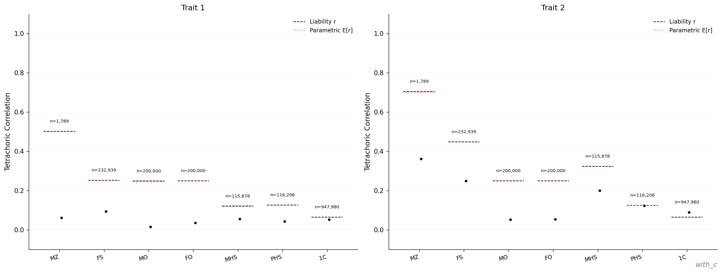
Comparison between trait 1 and trait 2

The relative-pair correlation page from results/examples/with_c/plots/atlas.pdf:

In simACE the C component is shared per household, where a household is defined by the mother (simace/simulation/simulate.py:761). Full siblings and maternal half-siblings therefore share C, whereas parents and their offspring, paternal half-siblings, and cousins draw C independently.

Class	Trait 1 (C=0)	Trait 2 (C=0.2)	Trait 2 expectation	Shares C?
MZ	0.50	0.70	\(v_A + v_C = 0.70\)	yes
FS	0.25	0.45	\(0.5\,v_A + v_C = 0.45\)	yes (same mother)
MO	0.25	0.25	\(0.5\,v_A = 0.25\)	no (different generation)
FO	0.25	0.25	\(0.5\,v_A = 0.25\)	no
MHS	0.125	0.325	\(0.25\,v_A + v_C = 0.325\)	yes (same mother)
PHS	0.125	0.125	\(0.25\,v_A = 0.125\)	no (different mothers)
1C	0.0625	0.0625	\(0.0625\,v_A = 0.0625\)	no

The variance-component checks in validation.yaml recover \((0.5, 0.0, 0.5)\) for trait 1 and \((0.5, 0.2, 0.3)\) for trait 2, in agreement with the configured inputs.

Observations

Observation 1 — C inflates only the relative classes that share a mother

MZ, FS, and MHS each gain exactly \(v_C = 0.2\) between trait 1 and trait 2; MO, FO, PHS, and 1C are unchanged. The increment is the same in every class that shares C, regardless of the additional contribution from the additive component, because the C component is shared in full or not at all.

Observation 2 — The MZ–FS gap is invariant to \(v_C\)

The difference \(r_{MZ} - r_{FS} = 0.5 \, v_A\) is independent of \(v_C\), because both MZ and FS share C in full and the \(v_C\) term cancels. Consequently, Falconer's formula \(2(r_{MZ} - r_{FS})\) estimates \(h^2\) rather than \(h^2 + c^2\), and both traits return \(\approx 0.5\) from Falconer despite their materially different relative-pair correlation patterns.

Observation 3 — The MHS–PHS contrast is a direct estimator of \(v_C\)

Maternal and paternal half-siblings share the same \(0.25 \, v_A\) by relatedness; the only structural difference between them in this model is that MHS share C and PHS do not. It follows that \(r_{MHS} - r_{PHS} = v_C\) exactly. The trait 2 panel gives \(0.325 - 0.125 = 0.20\), matching the configured input; the trait 1 panel gives \(0\), also as expected. This contrast is the identifiability condition that allows the ACE model to separate \(v_C\) from \(v_E\) (see the ACE Model concept page), and it relies on the maternal household structure used by simACE.

The case in which the clean C decomposition breaks — for example, under assortative mating, which moves variance into a covariance between mates — is treated in AM and Heritability.